Introduction

You probably tried using the Euler's method of estimating the next value of a function. Never heard of it? It goes something like this :

\[ \text{If we define a function }f(x)\text{ , and a infinitesimal difference }\Delta h\text{,}\]

\[\text{we can estimate }f(x+\Delta h)\approx f(x)+\Delta h*f'(x)\]

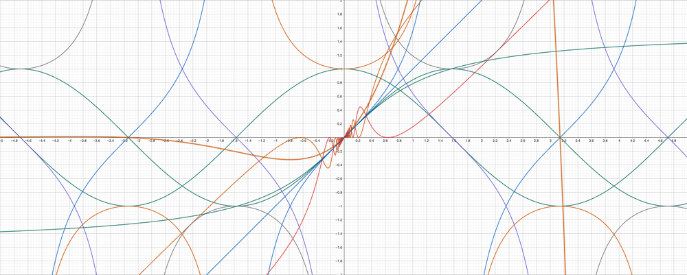
However, this method of estimation may not be correct at all times, especially if the function changes rapidly by x. For the simplicity of the explanation, lets assume there are two functions, \(y=sin(x)\) and \(y=x\) :

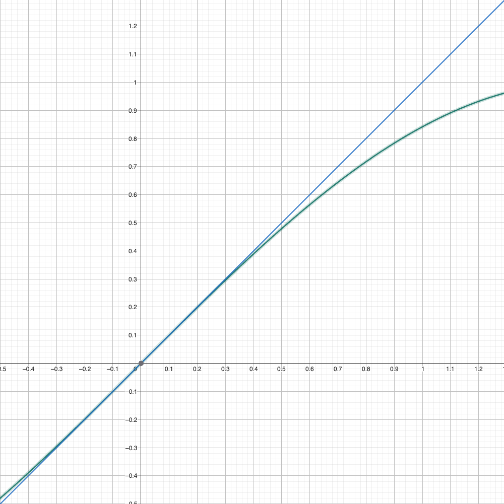
If we randomly assume that \(\Delta h=1\), we can find that error is already about \(0.15\). The error just gets worse as \(\Delta h\) increases. Of course, in this case, we can argue that h isn't infinitesimal, but what about functions like \(y= x+x\cdot sin(\frac{1}{x})\)?

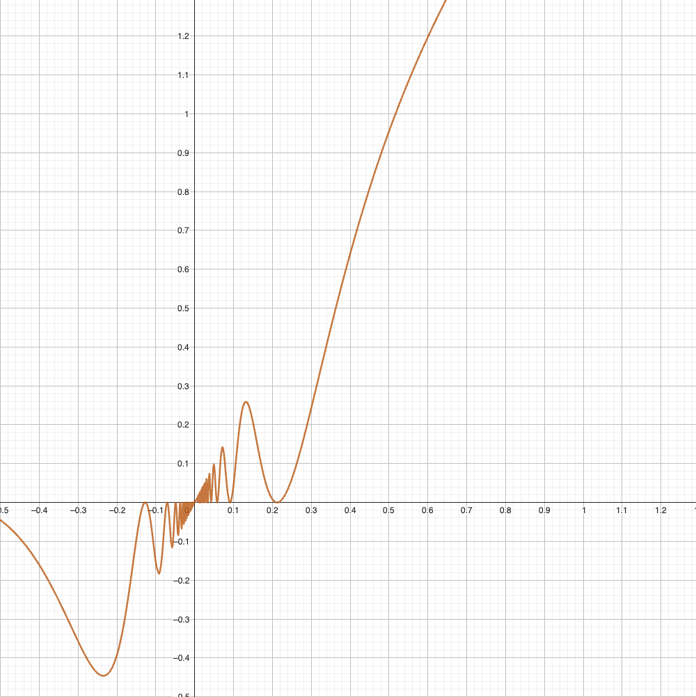
Here, using the Euler method isn't just good enough.

However, did you know there is a much better way of approximating this?

The R-K method, more well known as the Runge-Kutta method, is a powerful way to interpret Ordinary Differential Equations, or ODEs for short. To simplify, the R-K method is a more direct and precise way of estimating the next value of a function. One of it's greatest strengths is that it could be expanded infinitely, approaching \(0\) error.

However, it is extremely annoying to prove the R-K method by hand, since you would have to manually expand each element using the Taylor's Series(I'll make a post on this later. If you are interested right now, check out this video. ). Therefore, in this post, I'll prove the R-K 2 method, also known as the Improved Euler's Method or Heun's Method. This is much more easier, and the final form looks something like this :

\[ \text{DEFINITION}\]

\[ y'=f(x, y(x))\]

\[y_n=y(x_n)\text{, for the ease of proof}\]

\[ f_\alpha = \frac{\partial f}{\partial \alpha}\text{, for the ease of proof}\]

\[x_{n+1}= x_n+\Delta h\]

\[ \text{MAIN ALGORITHM}\]

\[k_1 = f(x_n, y_n)\]

\[k_2 = f(x_{n+1}, y_n+h\cdot k_1)\]

\[\text{Using the definition, we can know that} \]

\[ y_{n+1} = y_n+\frac{h}{2}(k_1+k_2)\]

Here, \(y'=f(x, y(x))\) shows that the derivative of the function \(y\) is defined by a certain state \(x\) and the value of the function \(y\) at that point. Now that we know what the R-K method(R-K 2 to be exact) looks like, lets prove it.

Proof

In the end, we can say that we are trying to find \(a_1\) and \(a_2\) where

\[ y_{n+1} = y_n+\frac{h}{2}(a_1 k_1+a_2 k_2)\]

Keeping this in mind, let's begin.

Step 1 : Expansion of \(y_{n+1}\) Using Taylor's Series

To begin the proof, we must expand \(y_{n+1}\) using Taylor's Series. This will look in the form :

\[ y_{n+1} = y_n+h\cdot y_n' + \frac{h^2}{2}\cdot y_n'' + O(h^3)\]

Here, \(O(h^3)\) signifies the error caused by the truncation of all terms after \(h^2\).

Here, it is trivial that \(y_n'=f(x_n, y_n)\). Let's mark this as \(y'=f\) for the ease of proof. You'll see why soon.

Okay, now let's write \(y_n''\) in terms of \(f\) and it's partial derivatives.

\[y_n'' = \frac{d}{dt}[f(x_n, y_n)]\]

\[=\frac{\partial}{\partial x}f(x_n, y_n) + \frac{\partial}{\partial y}f(x_n, y_n) \cdot \frac{dy}{dx}\]

\[=f_x+f_y\cdot f\]

Great! Now that we have \(y_n'\) and \(y_n''\) ready, we should compare this with the final form we created earlier.

Step 2 : Expansion of \(k_2\) Using Taylor's Series

In order to compare coefficients, we must express \(k_2\) in terms of \(f\) and it's partial derivatives, not \(k_1\). This is quite easy, since we already expanded a very similar-looking expression(we just did it in step 1).

\[k_2 = f(x_{n+1}, y_n+h\cdot k_1)\]

\[=f(x_{n+1}, y_n + h \cdot f(x_n, y_n))\]

\[=f + h \cdot [f_x+f_y\cdot f] + O(h^2)\]

\[=f + h \cdot f_x + h \cdot f \cdot f_y\]

Here, since there's a lot of functions appearing here, the entire process becomes very intuitive once you substitute \(\frac{\partial}{\partial \alpha}f(x_n, y_n) \) as \( f_{\alpha}\).

Now that we have \(k_1\) and \(k_2\) prepared, let's move on to the final step.

Step 3 : Comparison of Coefficients

Till this point, we have expressed various expressions in terms of \(f\) and it's partial derivatives. From this, we can now express \(y_{n+1}\) in two forms, from the Taylor's Series, and from the R-K method.

\[ y_{n+1} = \underbrace{y_n+\frac{h}{2}(a_1 k_1 + a_2 k_2)}_{\text{From R-K 2}}\]

\[ = \underbrace{ y_{n+1} = y_n+h\cdot y_n' + \frac{h^2}{2}\cdot y_n''}_{\text{From Taylor's Series}}\]

After plugging in the expressions for \(k_1\), \(k_2\), \(y_n'\), and \(y_n''\), we can find that

\[a_1+a_2 = 2\]

\[a_1 = 1\]

Pretty easy from this point, I guess. Therefore, we can find that \(a_1 = a_2 = 1\), thus proving the R-K 2 method.

Step 3 + \(\alpha\) : The Derivative of Multivariate Functions

This entire article is about finding the derivative of multivariate functions, or functions which receive multiple values as input. Specifically, in this case, we can define our case as :

\[ x : \text{a variable}\]

\[ y(x) : \text{a function which receives a variable x as input}\]

\[ f(x, y(x)): \text{a multivariate function}\]

To add a bit more, we can see that the second variable, \(y(x)\) is directly influenced by x.

To spill the beans before the actual proof, the derivative of the function \(f(x, y(x))\) can be expressed like the following :

\[ [f(x, y(x))]' = \frac{\partial}{\partial x}f(x, y(x)) + \frac{\partial}{\partial y}f(x, y(x)) \cdot \frac{dy}{dx}\]

OK, let's prove this. by the definition of derivatives, we know that

\[ \lim_{\Delta h\to\infty} f(x) = \frac{f(x+\Delta h, y(x+\Delta h)) - f(x, y(x))}{\Delta h} \]

Add and subtract \( f(x, y(x+h))\) to the numerator. The expression can be split into two parts :

\[ \lim_{\Delta h\to\infty}\underbrace{\frac{f(x+\Delta h, y(x+\Delta h)) - f(x, y(x+\Delta h))}{\Delta h}}_{\text{Part I}}\]

\[+ \underbrace{\frac{f(x, y(x+\Delta h)) - f(x, y(x))}{\Delta h}}_{\text{Part II}}\]

Part I can be easily expressed as \( \frac{\partial f}{\partial x}\). To find the derivative of part II, multiply \( y(x+\Delta h)-y(x)\) to both the numerator and the denominator. The expression, once simplified, can be expressed as :

\[ \frac{\partial f}{\partial y} \cdot \frac{dy}{dx}\]

Thus, the final equation becomes :

\[ [f(x, y(x))]' = \frac{\partial}{\partial x}f(x, y(x)) + \frac{\partial}{\partial y}f(x, y(x)) \cdot \frac{dy}{dx}\]

Conclusion

As stated in the introduction, the Runge-Kutta method is an extremly powerful method for estimating unknown future function values. This algorithm is utilized in various areas in science, and here are just a few :

• Projectile motion simulation with air resistance
• Planetary motion for N-planet systems
• Fluid dynamics
• Heat transfer
• And so much more....

Well, that's one more algorithm that's good to have in mind.