Introduction

In the last post, we dived into the basic terms and proofs for the Runge-Kutta method. In this post, let's explore the use of a Runge-Kutta method in a simple real-life stituation.

Let's begin!

A Quick Recap

The Runge-Kutta method(AKA the R-K method) is used for interpreting ordinary differential equations. Below is the basic form for a R-K 2 method :

\[ \text{DEFINITION}\]

\[ y'=f(x, y(x))\]

\[y_n=y(x_n)\text{, for the ease of proof}\]

\[ f_\alpha = \frac{\partial f}{\partial \alpha}\text{, for the ease of proof}\]

\[x_{n+1}= x_n+\Delta h\]

\[ \text{MAIN ALGORITHM}\]

\[k_1 = f(x_n, y_n)\]

\[k_2 = f(x_{n+1}, y_n+h\cdot k_1)\]

\[\text{Using the definition, we can know that} \]

\[ y_{n+1} = y_n+\frac{h}{2}(k_1+k_2)\]

We have proved in the previous post that the above equations hold for the definition above.

Spring, and More Springs!

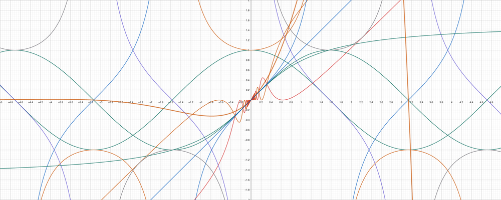
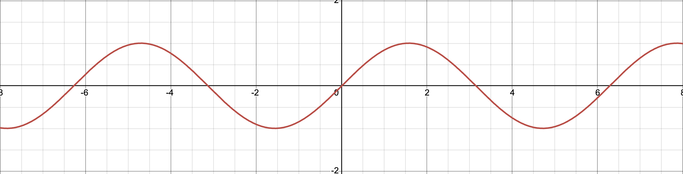
Let's imagine a basic spring oscillation. If there is no resistance, the location of the endpoint of the spring would follow that path of a trigonometric graph, somewhat similar to below :

For a more specific case, imagine a diagram like below where the large black dot is the fixed point :

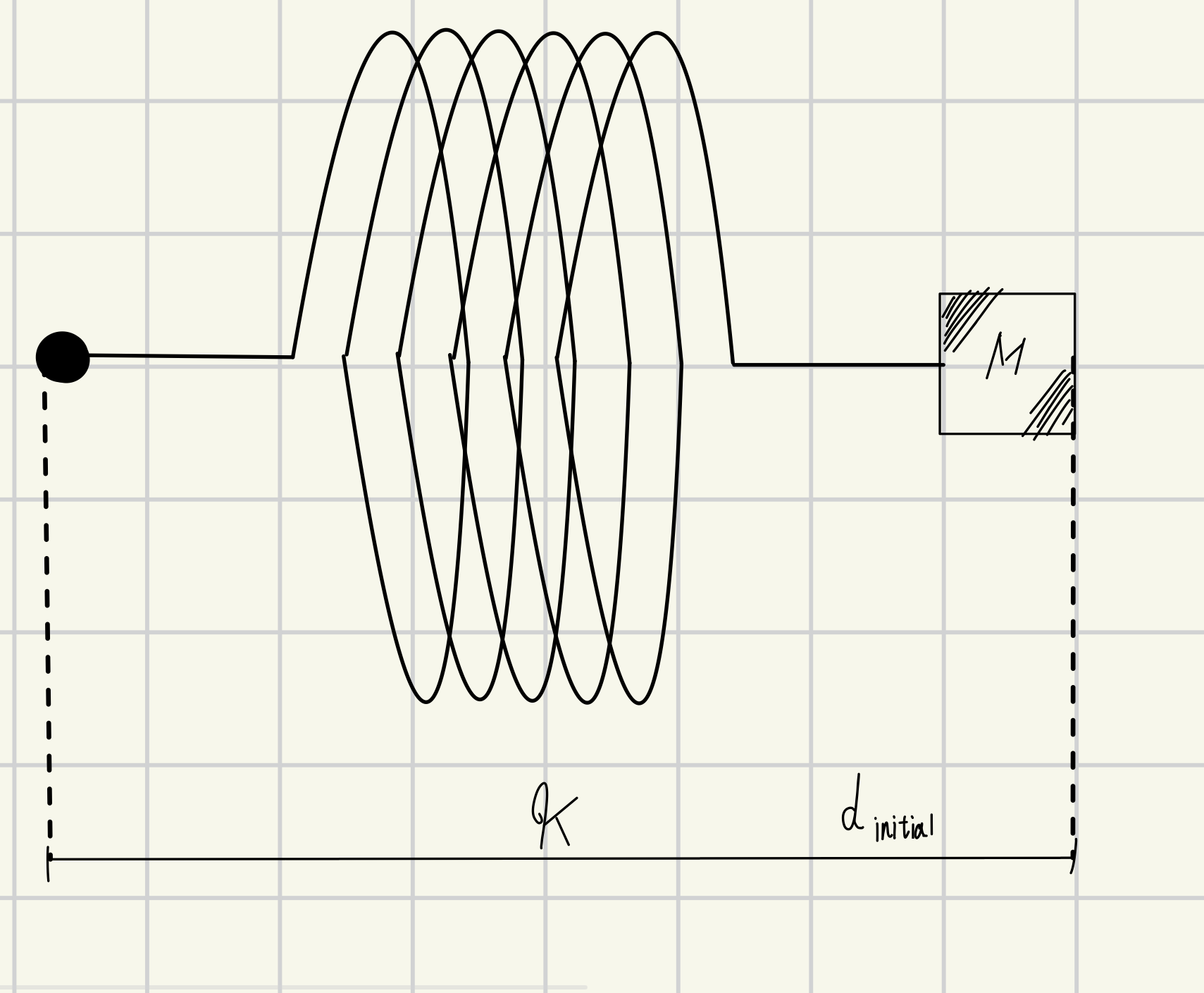
Let's define the values shows in the diagram as follows :

\[ \text{DEFINITION}\]

\[ \text{Define K as the spring constant of the given spring(N/m)}\]

\[ \text{Define } d_{initial} \text{ as the initial length of the setup(m)}\]

\[ \text{Define M as the mass of the weight attached to the other end of the spring}\]

\[ \text{relative to the fixed point. }\]

Understanding the diagram & Mathematical Proof

Let's test a standard case where \( K = 100N/m\), \(M = 1kg\), and \( d = 0.1m\). Since we have the needed physical knowledge to model this movement, let's use this to create a ideal simulation of the system.

\[\text{Let the displacement of the mass object at time t be y.}\]

\[\text{The formula for y is : }\]

\[y = d_{initial}\cos(\omega t)\]

\[\text{If we differentiate the equation above, we get : }\]

\[v = y' = -d_{initial} \omega\sin(\omega t)\]

\[\text{Differentiate again, }\]

\[a = v' = y'' = -d_{initial} \omega^2\cos(\omega t)\]

\[\text{Thus, }\]

\[a = -y\omega^2\]

\[\text{Multiplying both sides by M, }\]

\[F_{spring} = -My\omega^2\]

\[-Ky = -My\omega^2\]

\[K = M\omega^2\]

\[\therefore\omega = \sqrt{\frac{K}{M}}\]

\[\text{Using this info, we can easily calculate }\]

\[\text{that for this case, }\omega\text{ = 10 }\]

\[\therefore \text{Ideal Formula : }\]

\[y = 0.1\cos(10t)\]

Now that we have an ideal formula to model the oscillation of a string, let's code a simulation for this.

Simulation Time

In the simulation, we do not have access to the speed and position values of the object. Instead, we only have the ability to calculate the acceleration value at a given time point t and (estimated) displacement of the object. From this, we can know that we need to first find the speed data via the R-K method from the acceleration data, and then find the position data afterwards.

Below is the basic definitions for the simulation of oscillation. The accelerator function takes care of the accelerations that are exerted on the object, while the answerFunction function is designed to model an ideal oscillation of the system.

export class Oscillation {
    springConstant: number = 0;//in N/m
    mass: number = 0;//in kg
    amplitude: number = 0;
    omega: number = 0;

    constructor(mass, springConstant) {
        this.springConstant = springConstant;
        this.mass = mass;
        this.amplitude = this.mass * 10 / this.springConstant;
        this.omega = Math.sqrt(this.springConstant/this.mass);
    } 
    answerFunction = (t: number) => {
        return -this.amplitude*Math.sin(this.omega*t);
    }

    accelerator = (pos: Vector, rate: Vector) => {
        let posArr = pos.toArray()
        posArr = posArr.map(pi => {
            return - pi * this.springConstant / this.mass;
        });
        return new Vector(posArr);
    }
}

The main R-K region is actually two Runge-Kutta modules integrated into one; p1 relates to point 1 where k1 is calculated while p2 relates to point 2 where k2 is calculated. Since this code uses the Enhanced Euler's Method mentioned in part 1, the two points correspond to the original point and the point estimated by Euler's method.

export class RungeKutta2 {
    deltaH: number;//in seconds
    private readonly rateDerivativeFn: RateDerivativeFn;
    constructor(rateDerivativeFn: RateDerivativeFn, dH: number) {
        this.rateDerivativeFn = rateDerivativeFn;
        this.deltaH = dH
    }

    step(currentState: State): State {
        if(currentState.value.dim != currentState.rate.dim) {
            throw new Error(`Dimmensions do not match with Value: ${currentState.value.dim} vs Rate: ${currentState.rate.dim}`);
        }
        const p1value = currentState.value;
        const p1rate = currentState.rate;
        const p1rateDeriv = this.rateDerivativeFn(p1value, p1rate);

        const k1rate = p1rate;
        const k1rateDeriv = p1rateDeriv;

        const p2value = currentState.value.add(currentState.rate.scale(this.deltaH));
        const p2rate = currentState.rate.add(k1rateDeriv.scale(this.deltaH));
        const p2rateDeriv = this.rateDerivativeFn(p2value, p2rate)

        const k2rate = p2rate;
        const k2rateDeriv = p2rateDeriv;

        const nextValue = currentState.value.add(k1rate.scale(this.deltaH/2)).add(k2rate.scale(this.deltaH/2));
        const nextRate = currentState.rate.add(k1rateDeriv.scale(this.deltaH/2)).add(k2rateDeriv.scale(this.deltaH/2));
        return {value: nextValue, rate: nextRate};

    }
}

An Euler class was also created to compare against traditional methods.

export class Euler {

    deltaH: number;//in seconds
    private readonly rateDerivativeFn: RateDerivativeFn;

    constructor(rateDerivativeFn: RateDerivativeFn, deltaH: number) {
        this.rateDerivativeFn = rateDerivativeFn;
        this.deltaH = deltaH;
    }

    step(state: State): State {
        if (state.value.dim !== state.rate.dim) {
            throw new Error("Value and rate vectors must have the same dimension");
        }

        const rateDerivative = this.rateDerivativeFn(state.value, state.rate);

        const nextValue = state.value.add(state.rate.scale(this.deltaH));
        const nextRate  = state.rate.add(rateDerivative.scale(this.deltaH));

        return { value: nextValue, rate: nextRate };
    }
}

Results

Below is the graph that plots the estimated values for the position of the object after time t;

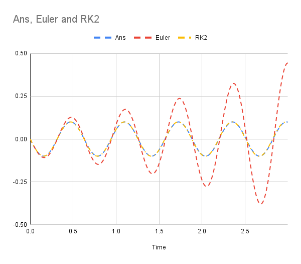
It doesn't take too much mathematical knowledge to find out that R-K 2 is so much better than Euler's method, in terms of correctness. To show more, here's a graph showing the errors of R-K 2 and Euler;

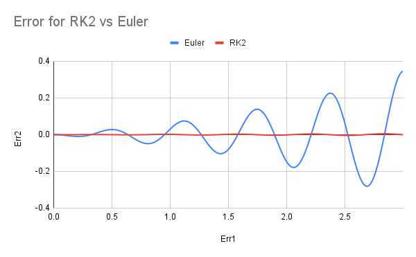
The error graph for the R-K 2 method stays on the x-axis while the error graph for Euler's method diverges.

Conclusion

Imagine simulating the path of a spaceship with the Euler's method. You would end up in Venus if you aimed for Mars. Not ideal.